The Skyquad
2015-09-15
A skyquad is to a quad what a skybox is to a box. The skyquad renders the sky by sending just a single quad down the rendering pipeline. The skyquad is useful not only in OpenGL, but also in ray tracing, where we have rays passing through an image plane. It was in this latter context where I first implemented a skyquad, so this post begins with the general mathematical machinery for a ray tracer and then applies it to OpenGL.
The Ray Equation
In a ray tracer, we have a camera and a window into the world - the image to be rendered - and we shoot rays passing through each the pixel of the image:

We can describe the problem of determining the ray through a given point in the image as follows:
Input:
- \(\vec{u}\), \(\vec{r}\), and \(\vec{f}\) - the camera’s up, right, and forward vectors, respectively.
- \(\vec{o}\) - the camera’s position.
- fovy - the camera’s vertical field of view angle.
- \((w,h)\) - the width and height of the image, respectively.
- \((x,y)\) - the coordinates of the target point in the image, ranging from \((0,0)\) to \((w,h)\).
Output:
- The ray \(r\) originating at \(\vec{o}\) and passing through \((x,y)\).
We adopt the following conventions:
- \((0,0)\) corresponds to the bottom-left corner of the image.
- \((w,h)\) corresponds to the top-right corner of the image.
Note that \((x,y)\) need not correspond with the integer coordinates of a pixel; it can be any real point on the image plane.
Determining the distance to the image plane
The first step is determining the distance \(d\) from the camera to the image plane, as shown in the image below:
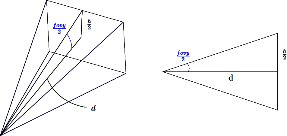
From the image, we can see that:
\[tan(\frac{fovy}{2}) = \frac{h/2}{d}\]
Solving for \(d\) yields:
\[\begin{align} tan(\frac{fovy}{2}) &= \frac{h/2}{d} \\\\ & \Leftrightarrow \\\\\ d &= \frac{h/2}{tan(\frac{fovy}{2})} \\\\ &= \frac{h}{2}\;cot(\frac{fovy}{2}) \end{align}\]h}{2};cot() \end{align}
Deriving the ray equation
Next, from the first figure, we can observe that the center of the image is determined by:
\[\vec{c} = \vec{o} + d\vec{f}\]
To reach the target point \((x,y)\) from \(\vec{c}\), we offset \(\vec{c}\) by a delta. We push \(\vec{c}\) \(d\_x\) units along the camera’s right vector \(\vec{r}\) and \(d\_y\) units along the camera’s up vector \(\vec{u}\):
\[[x,y] = \vec{c} + d\_x\vec{r} + d\_y\vec{u}\]
Deriving \(d\_x\) and \(d\_y\) is straightforward. When \(x=0\), \(d\_x=-w/2\), and when \(x=w\), \(d\_x=w/2\). The case for \(d\_y\) is similar. This results in:
\[d\_x = x - \frac{w}{2}\]
\[d\_y = y - \frac{h}{2}\]
The vector from the camera position \(\vec{o}\) to the point \((x,y)\) on the image plane is then given by:
\[\begin{align} \vec{v} &= [x,y] − \vec{o} \\\\ &= \vec{c} + d\_x\vec{r} + d\_y\vec{u} - \vec{o} \\\\ &= \vec{o} + d\vec{f} + d\_x\vec{r} + d\_y\vec{u} - \vec{o} \\\\ &= d\vec{f} + d\_x\vec{r} + d\_y\vec{u} \\\\ &= d\vec{f} + (x - \frac{w}{2})\vec{r} + (y - \frac{h}{2})\vec{u} \end{align}\]
Finally, the ray equation is \(r = \vec{o} + \lambda\vec{t}\), where \(\vec{t}\) is conveniently defined as \(\vec{v}\) normalised: \(\vec{t} = \frac{\vec{v}}{||\vec{v}||}\).
The Skyquad in OpenGL
To draw the skyquad in OpenGL, we render a quad directly in NDC space [1], with \(z=1\) to send it to the background. For each pixel in the quad, we compute the ray originating from the camera passing through that pixel. We then use the ray’s direction to sample a cubemap texture holding the skybox data. The fetched texel determines the colour value of the pixel.
To simplify our calculations, we compute the ray direction in NDC space and then apply the viewport’s aspect ratio \(r\) and the camera’s rotation matrix \(R\) to transform it into world space. NDC space has many interesting properties that make the calculations easier:
- \(\vec{u} = (0,1,0)\), \(\vec{r} = (1,0,0)\), and \(\vec{f} = (0,0,-1)\), assuming a right-handed coordinate system.
- \(\vec{o} = \vec{0}\)
- \(z\) = 1 (send quad to the background)
- \((w,h) = (1,1)\)
Using the properties above, the distance to the image plane \(d\) becomes:
\[\begin{align} d &= \frac{h}{2}\;cot(\frac{fovy}{2}) \\\\ &= \frac{1}{2}\;cot(\frac{fovy}{2}) \end{align}\]
The ray’s direction vector in NDC space is:
\[\begin{align} \vec{v}' &= d\vec{f} + (x - \frac{w}{2})\vec{r} + (y - \frac{h}{2})\vec{u} \\\\ &= d[0,0,-1] + (x - \frac{1}{2})[1,0,0] + (y - \frac{1}{2})[0,1,0] \\\\ &= [x - \frac{1}{2}, y - \frac{1}{2}, -d] \end{align}\]
Next, apply the viewport’s aspect ratio \(r\) to properly scale the ray:
\[v = v' * [r,1,1]\]
And finally, normalise the vector and apply the camera’s rotation matrix \(R\) to obtain the direction in world space:
\[\vec{t} = R \frac{\vec{v}}{||\vec{v}||}\]
To render the skyquad, we send a 2D quad with coordinates ranging from \((-1,-1)\) to \((1,1)\) down the pipeline with the shader program that follows. Please note the following implementation details:
- We do not need to compute a ray per pixel; instead, we can compute a ray for every vertex of the quad and let the pipeline interpolate the rays.
- Cubemap sampling does not require the vector to be normalized. Therefore, to make the shader more efficient, we do not normalize the sky ray.
Vertex shader
uniform mat3 Rotation;
uniform float fovy;
  uniform float aspect;

layout (location = 0) in vec2 Position;

out vec3 Ray;

vec3 skyRay (vec2 Texcoord)
{
    float d = 0.5 / tan(fovy/2.0);
    return vec3((Texcoord.x - 0.5) * aspect,
                 Texcoord.y - 0.5,
                 -d);
}

void main ()
{
    Ray = Rotation * skyRay(Position*0.5 + 0.5); // map [-1,1] -> [0,1]
    gl_Position = vec4(Position, 0.0, 1.0);
}
Fragment shader
uniform samplerCube tex;
in vec3 Ray;
layout (location = 0) out vec4 Colour;
void main ()
{
vec3 R = normalize(Ray);
Colour = vec4(pow(texture(tex, R).rgb, vec3(1.0/2.2)), 1.0);
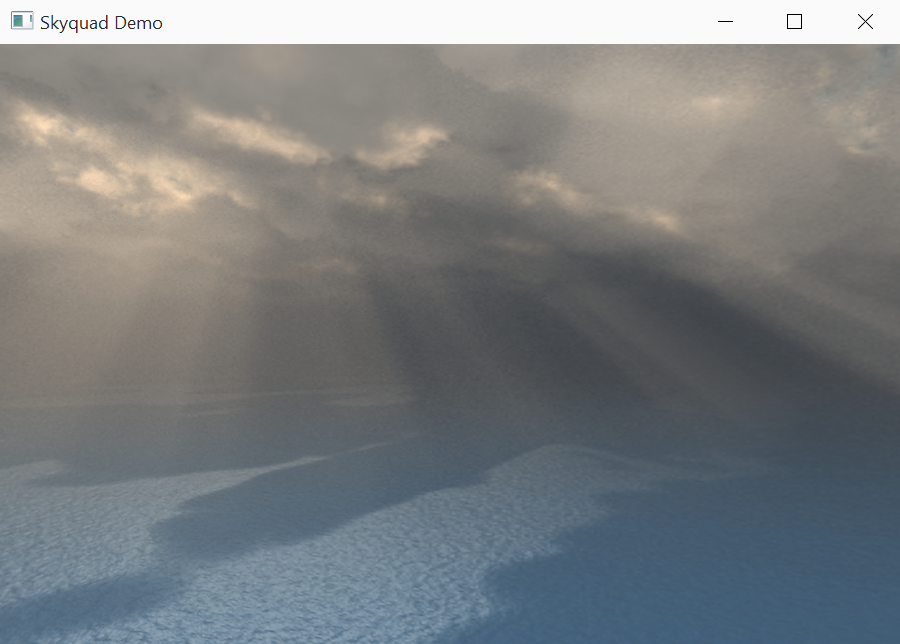
}Certainly a lot of maths for such a simple shader, but that is the beauty of computer graphics. The final solution is simple and works for both ray tracing and OpenGL. Below is a screenshot produced by a skyquad:
[1] Technically it is clip space, but since we set \(w=1\) in the shader then the perspective division leaves the coordinates unchanged.